SVM可视化问题以及概念问题
请问支持向量机数据中特征向量有多个,但可视化的时候是只能可视化其中的两个特征向量吗?
是的,支持向量机(Support Vector Machine,SVM)是一种二分类模型,其决策边界是一个超平面,而超平面的维度是数据特征空间的维度。因此,当数据特征向量的维度大于2时,我们无法直接在二维平面上对数据进行可视化。为了能够对数据进行可视化,我们通常会选择其中的两个特征向量,以二维平面上的坐标轴表示这两个特征向量,将其映射到二维平面上,然后用不同的符号或颜色来表示不同的类别,从而对数据进行可视化。这种方法通常被称为“二维投影”(2D projection),它虽然会丢失一部分数据的信息,但可以帮助我们更好地理解数据的特征和类别之间的关系。
你应该说的是维度吧,最多可以画出来3维。
- 这个问题的回答你可以参考下: https://ask.csdn.net/questions/1056427
- 我还给你找了一篇非常好的博客,你可以看看是否有帮助,链接:SVM解决回归问题
- 除此之外, 这篇博客: 【机器学习算法笔记系列】支持向量机(SVM)算法详解和实战中的 支持向量机实战—乳腺癌检测 部分也许能够解决你的问题, 你可以仔细阅读以下内容或跳转源博客中阅读:
本文使用支持向量机算法解决乳腺癌检测问题。
scikit-learn中自带一个乳腺癌数据集,为了方便起见,我们直接使用,读者也可直接在网上下载。乳腺癌数据集地址首先,我们加载数据,输出数据形状和特征。以查看数据:
__author__ = "fpZRobert" """ 支持向量机实战-乳腺癌检测 """ import warnings warnings.filterwarnings("ignore", category=FutureWarning, module="sklearn", lineno=196) from sklearn.datasets import load_breast_cancer """ 加载数据 """ cancer = load_breast_cancer() X = cancer.data y = cancer.target print("Shape of X: {0}; positive example: {1}; negative: {2}".format(X.shape, y[y==1].shape[0], y[y==0].shape[0])) # 查看数据的形状和类别分布 Out: Shape of X: (569, 30); positive example: 357; negative: 212我们可以看到,数据集总共有569个样本,每个样本有30个特征,其中357个阳性(y=1)样本,212个阴性(y=0)样本。之前在【机器学习算法笔记系列】逻辑回归(LR)算法详解和实战中详细介绍了数据集,这里不做过多描述,再一次介绍下10个特征:
特征 含义 radius 半径,即病灶中心点离边界的平均距离 texture 纹理,灰度值的标准偏差 perimeter 周长,即病灶的大小 area 面积,也是反映病灶大小的一个指标 smoothness 平滑度,即半径的变化幅度 compactness 密实度,周长的平方除以面积的商 concavity 凹度,凹陷部分轮廓的严重程度 concave points 凹点,凹陷轮廓的数量 symmetry 对称性 fractal dimension 分形维度 把数据集划分为训练集和测试集(划分比例一般80%用于训练,20%用于测试):
"""
    拆分数据集
"""
from sklearn.model_selection import train_test_split
X_train, X_test, y_train, y_test = train_test_split(X, y, test_size=0.2)
根据上述数据的介绍,我们的数据集很少,高斯核函数太复杂,容易造成过拟合,模型效果不会很好。为了验证我们的猜想,我们首先使用高斯核函数试着拟合数据,看下效果:
"""
    训练模型
"""
from sklearn.svm import SVC

clf = SVC(C=1.0, kernel="rbf", gamma=0.1)	# 使用高斯核函数
clf.fit(X_train, y_train)
train_score = clf.score(X_train, y_train)
test_score = clf.score(X_test, y_test)
print("train score: {0}; test score: {1}".format(train_score, test_score))

Out:
train score: 1.0; test score: 0.631578947368421
训练数据集评分接近满分,而交叉验证集评分很低,这是典型的过拟合现象。我们画出学习曲线,更加直观的看一下:
"""
    绘制学习曲线
"""
import numpy as np
import matplotlib.pyplot as plt
from sklearn.model_selection import ShuffleSplit
from sklearn.model_selection import learning_curve

# 绘制学习曲线
def plot_learning_curve(plt, estimator, title, X, y, ylim=None, cv=None,
                        n_jobs=1, train_sizes=np.linspace(.1, 1.0, 5)):
    plt.title(title)
    if ylim is not None:
        plt.ylim(*ylim)
    plt.xlabel("Training examples")
    plt.ylabel("Score")
    train_sizes, train_scores, test_scores = learning_curve(
        estimator, X, y, cv=cv, n_jobs=n_jobs, train_sizes=train_sizes)
    train_scores_mean = np.mean(train_scores, axis=1)
    train_scores_std = np.std(train_scores, axis=1)
    test_scores_mean = np.mean(test_scores, axis=1)
    test_scores_std = np.std(test_scores, axis=1)
    plt.grid()

    plt.fill_between(train_sizes, train_scores_mean - train_scores_std,
                     train_scores_mean + train_scores_std, alpha=0.1,
                     color="r")
    plt.fill_between(train_sizes, test_scores_mean - test_scores_std,
                     test_scores_mean + test_scores_std, alpha=0.1, color="g")
    plt.plot(train_sizes, train_scores_mean, 'o--', color="r",
             label="Training score")
    plt.plot(train_sizes, test_scores_mean, 'o-', color="g",
             label="Cross-validation score")

    plt.legend(loc="best")
    return plt

cv = ShuffleSplit(n_splits=10, test_size=0.2, random_state=0)
title = "Learning Curves for Gaussian Kernel"
plt.figure(figsize=(10, 4), dpi=144)
plot_learning_curve(plt, SVC(C=1.0, kernel="rbf", gamma=0.01), title, X, y, ylim=(0.5, 1.01), cv=cv)
plt.show()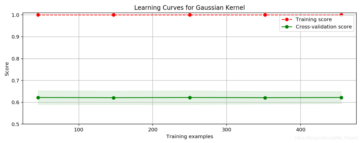
代码中gamma的参数选择为0.1,这个值相对已经很小了。通过上述参数介绍,我们知道gamma是核函数的系数(gamma值越小,支持向量越多)。我们试着利用之前讲过的GridSearchCV来自动选择参数:""" 模型调优 """ from sklearn.model_selection import GridSearchCV gammas = np.linspace(0, 0.0003, 30) param_grid = {"gamma": gammas} clf = GridSearchCV(SVC(), param_grid, cv=5) clf.fit(X, y) print(" best param: {0}\n best score: {1}".format(clf.best_params_, clf.best_score_)) Out: best score: 0.9367311072056239gamma是选择RBF函数作为kernel后,该函数自带的一个参数。隐含地决定了数据映射到新的特征空间后的分布,gamma越大,支持向量越少,gamma值越小,支持向量越多。支持向量的个数影响训练与预测的速度。通过GridSearchCV我们选择了最优gamma参数,交叉验证集的评分增加了不少,是不是此时的模型就是最好的呢?我们来换个模型,使用二阶多项式核函数来拟合模型,看看结果如何:""" 训练模型: 二阶多项式核函数 """ clf = SVC(C=1.0, kernel="poly", degree=2) clf.fit(X_train, y_train) train_score = clf.score(X_train, y_train) test_score = clf.score(X_test, y_test) print("train score: {0}; test score: {1}".format(train_score, test_score)) Out: train score: 0.9824175824175824; test score: 0.956140350877193从上述结果,可以看出效果比使用
RBF核函数效果要好。作为对比,我们画出一阶多项式核二阶多项式的学习曲线,观察数据的拟合情况:""" 绘制学习曲线 """ cv = ShuffleSplit(n_splits=5, test_size=0.2, random_state=0) title = "Learning Curves with degree={0}" degrees = [1, 2] plt.figure(figsize=(12, 4), dpi=144) for i in range(len(degrees)): plt.subplot(1, len(degrees), i+1) plot_learning_curve(plt, SVC(C=1.0, kernel="poly", degree=degrees[i]), title.format(degrees[i]), X, y, ylim=(0.8, 1.01), cv=cv) plt.show()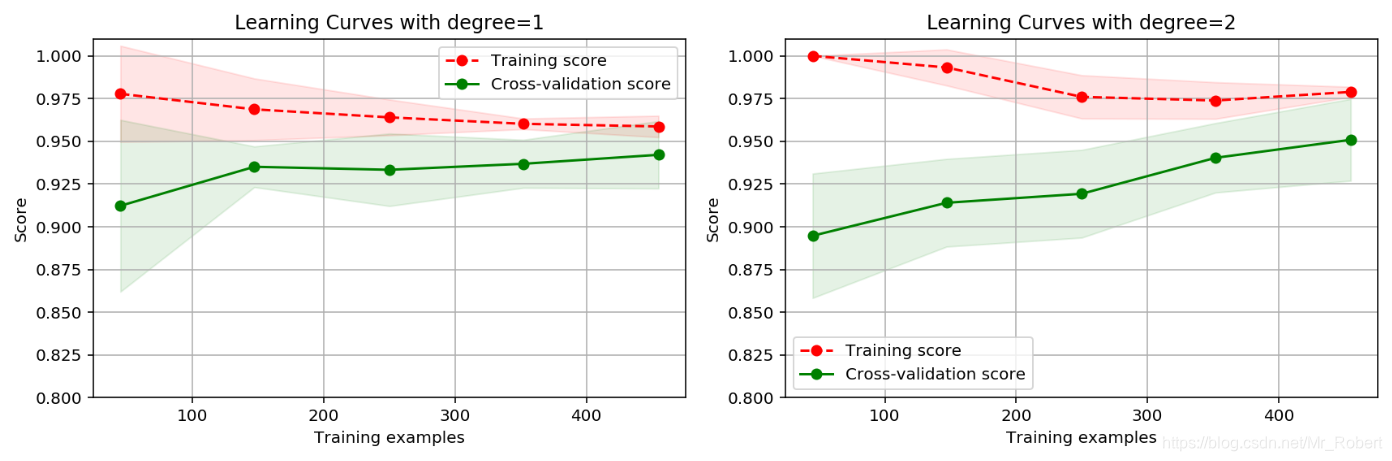
从图中可以看书,二阶多项式核函数的拟合效果更好。平均交叉验证集评分高达0.950,最高时达到0.975。运行该段代码需要注意,二阶多项式核函数计算代价很高,可能需要运行很长时间,请耐心等待结果。在之前的博客【机器学习算法笔记系列】逻辑回归(LR)算法详解和实战中,我们使用逻辑回归算法来进行乳腺癌的预测,使用二项多项式增加特征,同时使用
L1范数作为正则项,其拟合效果不仅比支持向量机好,而且在运算效率和计算代价上,远远好于二阶多项式核函数的支持向量机。当然,这里的支持向量机算法并未经过严谨的参数调优过程,但结果还是比使用L2范数的逻辑回归算法好,这里,我想表达的是:模型选择和参数调优,在工程实践中具有非常重要的作用。我们不仅需要掌握参数调优的科学方法,而且还需要了解各算法的适用场景和问题,以便选择最合适的算法模型去解决实际问题。全部代码:
# -*- coding: utf-8 -*-
# Time:2019/4/1 16:48
# versions:Python 3.6

__author__ = "fpZRobert"

"""
    支持向量机实战-乳腺癌检测
"""

import warnings
warnings.filterwarnings("ignore", category=FutureWarning, module="sklearn", lineno=196)

from sklearn.svm import SVC
import numpy as np
import matplotlib.pyplot as plt
from sklearn.model_selection import GridSearchCV
from sklearn.model_selection import ShuffleSplit
from sklearn.model_selection import learning_curve
from sklearn.datasets import load_breast_cancer
from sklearn.model_selection import train_test_split

"""
    加载数据
"""
cancer = load_breast_cancer()
X = cancer.data
y = cancer.target

print("Shape of X: {0}; positive example: {1}; negative: {2}".format(X.shape, y[y==1].shape[0], y[y==0].shape[0]))  # 查看数据的形状和类别分布

"""
    拆分数据集
"""
X_train, X_test, y_train, y_test = train_test_split(X, y, test_size=0.2)

"""
    训练模型: RBF核函数
"""

clf = SVC(C=1.0, kernel="rbf", gamma=0.1)
clf.fit(X_train, y_train)
train_score = clf.score(X_train, y_train)
test_score = clf.score(X_test, y_test)
print("train score: {0}; test score: {1}".format(train_score, test_score))

"""
    绘制学习曲线
"""

# 绘制学习曲线
def plot_learning_curve(plt, estimator, title, X, y, ylim=None, cv=None,
                        n_jobs=1, train_sizes=np.linspace(.1, 1.0, 5)):
    plt.title(title)
    if ylim is not None:
        plt.ylim(*ylim)
    plt.xlabel("Training examples")
    plt.ylabel("Score")
    train_sizes, train_scores, test_scores = learning_curve(
        estimator, X, y, cv=cv, n_jobs=n_jobs, train_sizes=train_sizes)
    train_scores_mean = np.mean(train_scores, axis=1)
    train_scores_std = np.std(train_scores, axis=1)
    test_scores_mean = np.mean(test_scores, axis=1)
    test_scores_std = np.std(test_scores, axis=1)
    plt.grid()

    plt.fill_between(train_sizes, train_scores_mean - train_scores_std,
                     train_scores_mean + train_scores_std, alpha=0.1,
                     color="r")
    plt.fill_between(train_sizes, test_scores_mean - test_scores_std,
                     test_scores_mean + test_scores_std, alpha=0.1, color="g")
    plt.plot(train_sizes, train_scores_mean, 'o--', color="r",
             label="Training score")
    plt.plot(train_sizes, test_scores_mean, 'o-', color="g",
             label="Cross-validation score")

    plt.legend(loc="best")
    return plt

cv = ShuffleSplit(n_splits=10, test_size=0.2, random_state=0)
title = "Learning Curves for Gaussian Kernel"
plt.figure(figsize=(10, 4), dpi=144)
plot_learning_curve(plt, SVC(C=1.0, kernel="rbf", gamma=0.01), title, X, y, ylim=(0.5, 1.01), cv=cv)
plt.show()

"""
    模型调优
"""

gammas = np.linspace(0, 0.0003, 30)
param_grid = {"gamma": gammas}
clf = GridSearchCV(SVC(), param_grid, cv=5)
clf.fit(X, y)
print("best param: {0}\n best score: {1}".format(clf.best_params_, clf.best_score_))

"""
    训练模型: 二阶多项式核函数
"""
clf = SVC(C=1.0, kernel="poly", degree=2)
clf.fit(X_train, y_train)
train_score = clf.score(X_train, y_train)
test_score = clf.score(X_test, y_test)
print("train score: {0}; test score: {1}".format(train_score, test_score))

"""
    绘制学习曲线
"""
cv = ShuffleSplit(n_splits=5, test_size=0.2, random_state=0)
title = "Learning Curves with degree={0}"
degrees = [1, 2]
plt.figure(figsize=(12, 4), dpi=144)
for i in range(len(degrees)):
    plt.subplot(1, len(degrees), i+1)
    plot_learning_curve(plt, SVC(C=1.0, kernel="poly", degree=degrees[i]), title.format(degrees[i]), X, y, ylim=(0.8, 1.01), cv=cv)
plt.show()