matlab程序无误,但是结果图没有出
```clear; close all;
%传递函数形式描述线性系统
b =[1];a =[1 3 2];
%转换成状态方程模型描述系统
[a,b,c,d]= tf2ss(b,a);
sys = ss(a,b,c,d);
t =0:0.1:10;
f = exp( - t); %输入信号
f0 =[2;0]; %初始状态
y1 = step(sys,t); %求单位阶跃响应
y2 = initial(sys,f0,t); %求零输入响应
function dydt = dydtfun(t,y)
dydt = zeros(2,1);% dydt(1) 表示,dydt 本身仅是普通变量
dydt(y1) = y2;% dydt(2) 表示
dydt(y2) = -3* y2 -2* y+ exp( - t);
t0 =0;tf =10;
[t,y]= ode45(' dydtfun' ,[t0,tf],[0;2]);% [0;2]是初始条件参数,表示 =0,=2
subplot(1,2,1),plot(t,y(:,1));grid on;
plot(t,y)
title('y(t)') ;
subplot(1,2,2),plot(t,y(:,2));grid on;
title('y/prime(t)') ;
end

如果要subplot,那么可以这么做
% 传递函数形式描述线性系统
b =[1];
a =[1 3 2];
%转换成状态方程模型描述系统
[a,b,c,d]= tf2ss(b,a);
sys = ss(a,b,c,d);
t =0:0.1:10;
f = exp( - t); %输入信号
f0 =[2;0]; %初始状态
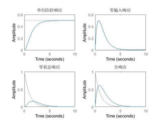
figure(1);clf
subplot(2,2,1)
step(sys,t); %求单位阶跃响应
title('单位阶跃响应')
subplot(2,2,2)
initial(sys,f0,t); %求零输入响应
title('零输入响应')
subplot(2,2,3)
lsim(sys, f,t);
title('零状态响应')
subplot(2,2,4)
lsim(sys, f,t, f0);
title('全响应')