)将一分一段表 分数段为 463-582 的数据按照组距为 8,借助 python 绘制频率分布直方图和直方图的外廓 曲线(概率密度曲线)
)将一分一段表 分数段为 463-582 的数据按照组距为 8,借助 python 绘制频率分布直方图和直方图的外廓
曲线(概率密度曲线)
- 你可以看下这个问题的回答https://ask.csdn.net/questions/7526462
- 这篇博客也不错, 你可以看下菜鸟写Python-数据库入门:通过7步曲掌握数据库的使用原理
- 除此之外, 这篇博客: Python计算机视觉-仿射扭曲简单实例中的 1.1 图像中的图像 部分也许能够解决你的问题, 你可以仔细阅读以下内容或跳转源博客中阅读:
放置图像的过程中,使用 warp.py 文件中的 image_in_image() 函数可以将目标图像中的角点坐标作为输入参数将第一幅扭曲后的图像与目标图像融合成了 Alpha 图像,扭曲的图像是在扭曲区域边界之外用 0 填充的图像,因此可以得到放置后的覆盖效果,而当前我们处理过程中的角点坐标是通过查看绘制好的图像人为手工确定的。
Alpha是一个8位的灰度图像通道,该通道用256级灰度来记录图像中的透明度信息,定义透明、不透明和半透明区域,其中黑表示透明,白表示不透明,灰表示半透明。
代码如下:
 # -*- coding: utf-8 -*-
from PCV.geometry import warp, homography
from PIL import Image
from pylab import *
from scipy import ndimage

# example of affine warp of im1 onto im2

im1 = array(Image.open('./images/1.jpg').convert('L'))
im2 = array(Image.open('./images/2.jpg').convert('L'))
# set to points
tp = array([[800, 1400, 1400, 800], [450, 450, 750, 800], [1, 1, 1, 1]])
#tp = array([[675,826,826,677],[55,52,281,277],[1,1,1,1]])
im3 = warp.image_in_image(im1, im2, tp)
figure()
gray()
# subplot(141)
# axis('off')
imshow(im1)
# subplot(142)
# axis('off')
figure()
imshow(im2)
# subplot(143)
# axis('off')
figure()
imshow(im3)
warp.py 当中的 image_in_image() 函数如下:
def image_in_image(im1,im2,tp):
    """ Put im1 in im2 with an affine transformation
        such that corners are as close to tp as possible.
        tp are homogeneous and counter-clockwise from top left. """

    # points to warp from
    m,n = im1.shape[:2]
    fp = array([[0,m,m,0],[0,0,n,n],[1,1,1,1]])

    # compute affine transform and apply
    H = homography.Haffine_from_points(tp,fp)
    im1_t = ndimage.affine_transform(im1,H[:2,:2],(H[0,2],H[1,2]),im2.shape[:2])
    alpha = (im1_t > 0)

    return (1-alpha)*im2 + alpha*im1_t
原书中的代码在我的环境中直接运行会出现报错:
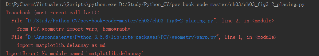
要将 warp.py 中首行导入语句修改为:from scipy.spatial import Delaunay
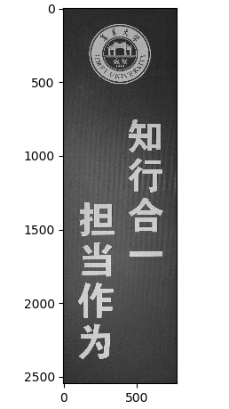
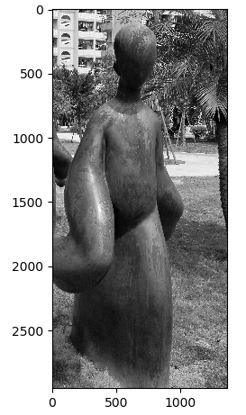
(上述代码中已修改)使用的两张原图:
融合后的结果: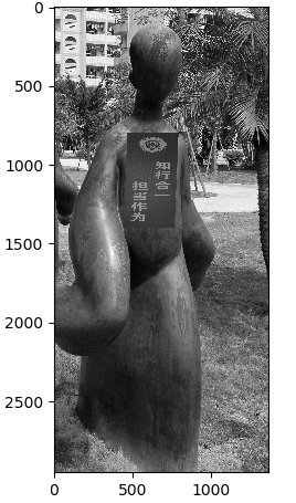
代码 image_in_image() 函数中:
shape 方法的功能是读取矩阵的长度,比如shape[0]就是读取矩阵第一维度的长度。它的输入参数可以使一个整数表示维度,也可以是一个矩阵。
Haffine_from_points() 会返回给定对应点对的最优仿射变换,适用于透视效应比较弱的情况下。- 以下回答由chatgpt基于相关博客总结生成:
我可以使用Python中的matplotlib库来绘制频率分布直方图和直方图的外廓曲线。具体步骤如下:
- 首先,需要准备数据集。根据题目提供的数据范围和组距,可以生成一个频率分布表。假设设定的组距为8,数据范围为[463, 582],则频率分布表如下:
区间 频数 463-470 0 471-478 1 479-486 2 487-494 3 495-502 4 503-510 5 511-518 6 519-526 7 527-534 8 535-542 9 543-550 10 551-558 11 559-566 12 567-574 13 575-582 14 - 将频率分布表转化为一个list,其中每个元素表示该区间的频数。代码如下:
freq_list = [0, 1, 2, 3, 4, 5, 6, 7, 8, 9, 10, 11, 12, 13, 14]
- 使用matplotlib库中的bar函数绘制频率分布直方图。需要设置好x轴和y轴的标签、标题等。代码如下:
import matplotlib.pyplot as plt
x = range(len(freq_list)) label = ['463-470', '471-478', '479-486', '487-494', '495-502', '503-510', '511-518', '519-526', '527-534', '535-542', '543-550', '551-558', '559-566', '567-574', '575-582'] plt.bar(x, freq_list, tick_label=label) plt.title('Frequency Distribution Histogram') plt.xlabel('Interval') plt.ylabel('Frequency') plt.show()
- 绘制直方图的外廓曲线需要进行插值。可以使用scipy库中的interp函数进行插值。代码如下:
import numpy as np from scipy.interpolate import interp1d
x = np.linspace(min(x), max(x), num=100, endpoint=True) f = interp1d(range(len(freq_list)), freq_list, kind='cubic') y = f(x)
- 最后,将插值结果绘制在直方图上,即可得到直方图的外廓曲线。需要设置好线条的颜色和线宽等。代码如下:
plt.plot(x, y, color='r', linewidth=2) plt.show()
完整代码如下:
import numpy as np from scipy.interpolate import interp1d import matplotlib.pyplot as plt
freq_list = [0, 1, 2, 3, 4, 5, 6, 7, 8, 9, 10, 11, 12, 13, 14]
x = range(len(freq_list)) label = ['463-470', '471-478', '479-486', '487-494', '495-502', '503-510', '511-518', '519-526', '527-534', '535-542', '543-550', '551-558', '559-566', '567-574', '575-582'] plt.bar(x, freq_list, tick_label=label) plt.title('Frequency Distribution Histogram') plt.xlabel('Interval') plt.ylabel('Frequency')
x = np.linspace(min(x), max(x), num=100, endpoint=True) f = interp1d(range(len(freq_list)), freq_list, kind='cubic') y = f(x)
plt.plot(x, y, color='r', linewidth=2)
plt.show()