图像能量图怎么计算,代码 matlab
图像能量图怎么计算,代码 matlab ,python也可以,但是要运行正确
MATLAB
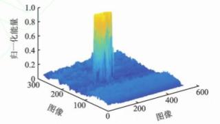
能量计算方式,直接取平方,你可以根据自己的计算方式进行更改
close all;
clear all;
A = imread('lena.png'); %换成自己的图
GRAY_A = double(rgb2gray(A))./255;
ENG_GRAY_A=GRAY_A.*GRAY_A;%计算能量
[x1,y1] = size(ENG_GRAY_A);
X = 0:x1-1;
Y = 0:y1-1;
figure
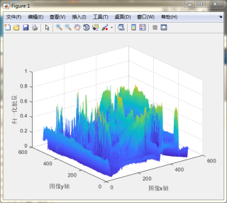
mesh(X,Y,ENG_GRAY_A)
xlabel('图像x轴');
ylabel('图像y轴');
zlabel('归一化能量');
matlab
能量= sum(abs(details(:)).^2);
 x = rand(64,64,16);
    J = 1;
    [Faf, Fsf] = FSfarras;
    [af, sf] = dualfilt1;T=10;
    w = dualtree3D(x, J, Faf, af);
    details = w{1}{1}{1};
    energy = sum(abs(details(:)).^2);
用surface
用python实现的:
import pandas as pd
import numpy as np
import matplotlib.pyplot as plt
import pywt
from mpl_toolkits.mplot3d import axes3d
from matplotlib.ticker import multiplelocator, formatstrformatter
# 解决负号显示问题
plt.rcparams['axes.unicode_minus'] = false  # 解决保存图像是负号'-'显示为方块的问题
plt.rcparams.update({'text.usetex': false, 'font.family': 'serif', 'font.serif': 'cmr10', 'mathtext.fontset': 'cm'})
font1 = {'family': 'simhei', 'weight': 'normal', 'size': 12}
font2 = {'family': 'times new roman', 'weight': 'normal', 'size': 18}
label = {'family': 'simhei', 'weight': 'normal', 'size': 15}
xlsx_path = "../小波能量谱作图.xlsx"
sheet_name = "表名"
data_arr = pd.read_excel(xlsx_path, sheet_name=sheet_name)
column_name = '列名'
row = 1024
y = data_arr[column_name][0:row]
x = data_arr['time'][0:row]
scale = np.arange(1, 50)
wavelet = 'gaus1'   # 'morl'  'gaus1'  小波基函数
# 时间-尺度小波能量谱
def time_scale_spectrum():
    coefs, freqs = pywt.cwt(y, scale, wavelet)  # np.arange(1, 31) 第一个参数必须 >=1     'morl'  'gaus1'
    scale_freqs = np.power(freqs, -1)  # 对频率freqs 取倒数变为尺度
    fig = plt.figure(figsize=(5, 4))
    ax = axes3d(fig)
    # x:time   y:scale   z:amplitude
    x = np.arange(0, row, 1)  # [0-1023]
    y = scale_freqs
    x, y = np.meshgrid(x, y)
    z = abs(coefs)
    # 绘制三维曲面图
    ax.plot_surface(x, y, z, rstride=1, cstride=1, cmap='rainbow')
    # 设置三个坐标轴信息
    ax.set_xlabel('$mileage/km$', color='b', fontsize=12)
    ax.set_ylabel('$scale$', color='g', fontsize=12)
    ax.set_zlabel('$amplitude/mm$', color='r', fontsize=12)
    plt.draw()
    plt.show()
# 时间小波能量谱
def time_spectrum():
    coefs, freqs = pywt.cwt(y, scale, wavelet)
    coefs_pow = np.power(coefs, 2)      # 对二维数组中的数平方
    spectrum_value = [0] * row    # len(freqs)
    # 将二维数组按照里程叠加每个里程上的所有scale值
    for i in range(row):
        sum = 0
        for j in range(len(freqs)):
            sum += coefs_pow[j][i]
        spectrum_value[i] = sum
    fig = plt.figure(figsize=(7, 2))
    line_width = 1
    line_color = 'dodgerblue'
    line_style = '-'
    t1 = fig.add_subplot(1, 1, 1)
    t1.plot(x, spectrum_value, label='模拟', linewidth=line_width, color=line_color, linestyle=line_style)
    # t1.legend(loc='upper right', prop=font1, frameon=true)  # lower ,left
    # 坐标轴名称
    t1.set_xlabel('$time$', fontsize=15, fontdict=font1)  # fontdict设置子图字体
    t1.set_ylabel('$e/mm^2$', fontsize=15, fontdict=font1)
    # 坐标刻度值字体大小
    t1.tick_params(labelsize=15)
    print(spectrum_value[269])
    plt.show()
# 尺度小波能量谱
def scale_spectrum():
    coefs, freqs = pywt.cwt(y, scale, wavelet)
    coefs_pow = np.power(coefs, 2)      # 对二维数组中的数平方
    scale_freqs = np.power(freqs, -1)   # 对频率freqs 取倒数变为尺度
    spectrum_value = [0] * len(freqs)    # len(freqs)
    # 将二维数组按照里程叠加每个里程上的所有scale值
    for i in range(len(freqs)):
        sum = 0
        for j in range(row):
            sum += coefs_pow[i][j]
        spectrum_value[i] = sum
    fig = plt.figure(figsize=(7, 4))
    line_width = 1
    line_color1 = 'dodgerblue'
    line_style1 = '-'
    t1 = fig.add_subplot(1, 1, 1)
    t1.plot(scale_freqs, spectrum_value, label=column_name, linewidth=line_width, color=line_color1, linestyle=line_style1)
    # t1.legend(loc='upper right', prop=font1, frameon=true)  # lower ,left
    # 坐标轴名称
    t1.set_xlabel('$scale$', fontsize=15, fontdict=font1)  # fontdict设置子图字体
    t1.set_ylabel('$e/mm^2$', fontsize=15, fontdict=font1)
    # 坐标刻度值字体大小
    t1.tick_params(labelsize=15)
    plt.show()
# 通过调用下面三个不同的函数选择绘制能量谱
time_scale_spectrum()
# time_spectrum()
# scale_spectrum()